Inside Hypercore: How TimescaleDB Quietly Built a Hybrid OLTP/OLAP Engine on Postgres
Disclosure: I work at Tiger Data, the company behind TimescaleDB. This post is my own analysis based on public documentation and code, and is not an official Tiger Data publication. I've tried to write the post I would have wanted to read six months ago.
The reframe
Here's something most people miss: Hypercore isn't a new feature. It's a rename.
The hybrid row-columnar storage engine inside TimescaleDB already existed — it was the machinery behind what everyone called "compression." Tiger Data renamed the whole package to Hypercore because they realized the conversion from row-oriented to column-oriented storage was what customers actually cared about. Compression was the side effect. Real-time analytics on fresh data was the prize.
That shift in framing matters. If you came to TimescaleDB looking for a time-series database with nice storage savings, you were buying the wrong thing. What you actually got was a Postgres extension that fuses an OLTP-style rowstore with an OLAP-style columnstore behind a single SQL surface — with no separate analytics database, no ETL, no eventual consistency.
This post is about how that actually works. Not the marketing version. The version where we look at chunks, catalogs, and compression algorithms, and ask: why does this work, and where does it break?
The two-store mental model
If you've worked with Postgres long enough, you already have the mental model for Hypercore — you just don't know it yet.
Think of how Postgres treats a freshly-inserted row versus an old one that's been vacuumed, frozen, and is sitting in a cold page on disk. Both are "the same table," but they live in different states, have different access patterns, and respond to different optimizations. Hypercore takes that idea and makes it explicit.
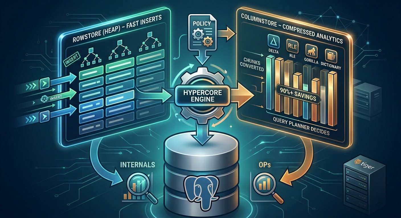
There are two stores:
The rowstore is regular Postgres heap storage. New data lands here. Inserts are fast. Updates and deletes work normally. Indexes behave the way you expect. If you stopped here, you'd just have a normal hypertable.
The columnstore is what older chunks get converted into. Each column is stored separately, compressed, and organized for scanning rather than point lookups. Aggregations fly. Scans skip irrelevant chunks entirely. Storage drops by 90–98%.
The trick is that both stores belong to the same hypertable. You don't query them separately. You write one SQL statement, and the planner figures out which chunks live where and reads accordingly. From the application's perspective, it's just a table.
-- This query reads transparently across rowstore and columnstore chunks
SELECT time_bucket('1 hour', ts) AS hour,
       device_id,
       avg(temperature)
FROM sensor_readings
WHERE ts > now() - INTERVAL '7 days'
GROUP BY hour, device_id;
The fresh chunks (last few hours) sit in the rowstore. The week-old chunks have been converted to the columnstore. You wrote one query. Postgres did the right thing.
What actually happens during conversion
Let's get concrete. A chunk's lifecycle looks like this:
Create the hypertable. You write a normal CREATE TABLE, then SELECT create_hypertable(...). TimescaleDB partitions the table into chunks based on a time interval (default: 7 days, configurable per workload).
Inserts hit the rowstore. Every INSERT lands in the chunk corresponding to its timestamp. These chunks are regular heap tables — Postgres doesn't know they're special. You can \d+ them.
A columnstore policy is configured. When you enable the columnstore on a hypertable, you tell TimescaleDB when chunks should convert (e.g., "after they're 7 days old") and how they should be organized (the segmentby and orderby options, which we'll get to).
ALTER TABLE sensor_readings SET (
  timescaledb.enable_columnstore = true,
  timescaledb.segmentby = 'device_id',
  timescaledb.orderby = 'ts DESC'
);SELECT add_columnstore_policy('sensor_readings', after => INTERVAL '7 days');
A background job converts old chunks. When a chunk crosses the age threshold, a background worker rewrites it. Rows get reorganized into column-major layout, compression algorithms run per column, and the result lands in internal storage that the hypertable knows how to read.
The original chunk is replaced. From a query planner perspective, the chunk is now "in the columnstore." It still belongs to the hypertable, still participates in queries, but is read through different machinery.
Modifications still work. This is the part that distinguishes Hypercore from a pure columnar engine. You can INSERT into a columnstore chunk, UPDATE it, DELETE from it. The engine handles the decompress-modify-recompress dance under transactional semantics. It's not free — there's overhead — but it works, which most columnar systems can't say.
If you want to see what's happening under the hood, the catalog views are your friend:
-- See which chunks are in the columnstore
SELECT chunk_schema, chunk_name, is_compressed
FROM timescaledb_information.chunks
WHERE hypertable_name = 'sensor_readings'
ORDER BY range_start DESC;-- See compression stats
SELECT pg_size_pretty(before_compression_total_bytes) AS before,
       pg_size_pretty(after_compression_total_bytes)  AS after
FROM hypertable_compression_stats('sensor_readings');
The compression algorithms (or: why your time-series data wants to be small)
Generic compression — gzip, LZ4, zstd — treats your data as an opaque stream of bytes. Time-series data isn't opaque. It has structure: timestamps tick forward at predictable intervals, sensor readings drift slowly, device IDs repeat for hours. A type-aware compressor can exploit that, and it's the difference between 3x and 30x ratios.
Hypercore picks the right algorithm per column type and layers them:
| Column type | Algorithm(s) | Why it works |
|---|---|---|
| Timestamps | Delta-of-delta + Simple-8b | Regular intervals → second derivative is zero → store almost nothing |
| Slow-moving floats | Gorilla XOR (Facebook's Gorilla paper) | Consecutive values share most bits; XOR leaves near-zero residual |
| Low-cardinality strings | Dictionary + RLE | Repeated values collapse to a count |
| Any small-integer stream | Simple-8b | Packs multiple values into one 64-bit word |
A timestamp column compressed with delta-of-delta + simple-8b gets to a few bits per row. A
status TEXT column with five distinct values across a billion rows costs essentially nothing. The cumulative layering is where the 90–98% numbers come from.What you control is the column layout — segmentby and orderby — which determines how much repetition each algorithm has to work with. Get those right and the compression engine does its job. Get them wrong and you'll wonder why your "compressed" data is still big.
segmentby and orderby: the two decisions that determine everything
If you remember nothing else from this post, remember this: the compression ratio you get is mostly a function of two settings. Not the algorithms, not the chunk size, not the hardware. Those two settings.
segmentby
segmentby tells the columnstore which columns to group rows by within a chunk. Think of it like a GROUP BY for storage: all rows with the same segmentby value get co-located, then compressed together.
Pick the right column and the compression algorithms see long runs of repeated values — RLE crushes them, dictionary encoding hands them off as a single integer, the column collapses to almost nothing. Pick the wrong column (or none at all) and the compressor sees a random salad of values and does its best, which isn't much.
Rule of thumb: segmentby should be the column you most often filter on, typically a low-to-medium cardinality identifier — device_id, tenant_id, symbol, host. Not a timestamp. Not a high-cardinality UUID. Not the metric value itself.
orderby
orderby controls the row order within each segment. The default is your time column descending, which is almost always right, but you can layer in additional columns.
Why does this matter? Because compression algorithms exploit locality. Delta-of-delta only works if consecutive rows have similar timestamps. Gorilla XOR only works if consecutive floats are similar. If your rows are in random order, none of that lands.
An example with numbers
Imagine a metrics table: (ts, device_id, temperature, humidity), one billion rows, 10,000 devices, one reading per minute per device.
| Configuration | Approximate ratio | Why |
|---|---|---|
No segmentby, no orderby | ~5x | Generic per-column compression, no locality |
segmentby = device_id, default orderby | ~25x | Per-device rows colocated, timestamps regular, floats drift slowly |
segmentby = device_id, ts (wrong) | ~3x | High-cardinality segments → tiny groups → no compression headroom |
These are illustrative ranges, not benchmarks — your data will vary. But the shape is real: a smart
segmentby is the difference between "TimescaleDB saved us a lot of money" and "we don't really see why people talk about this."To choose: find the column in the WHERE clause of 80% of your analytical queries, verify it has low-to-medium cardinality (aim for at least a few thousand rows per segment), then check hypertable_compression_stats after setup. If you're under 10x, your segmentby is wrong.
The OLTP problem (and what 2.18 did about it)
For most of Hypercore's life, there was one big asterisk: once a chunk moved to the columnstore, you lost your indexes.
This is the classic columnar-database problem. Column stores are great for "scan a billion rows and aggregate," terrible for "find the one row where transaction_id = 0xdeadbeef." Postgres's B-tree indexes — the things that make point lookups instant — don't translate naturally to compressed columnar layouts.
In practice, that meant: as soon as your data got compressed, looking up a single record turned into a sequential scan over the chunk. Updating a single sensor reading from three months ago became a "decompress the whole batch, modify, recompress" operation. Fine for analytics. Painful for hybrid OLTP/OLAP workloads where someone occasionally needs to correct a specific record.
TimescaleDB 2.18 fixed this. B-tree and hash indexes now work on columnstore chunks (still labeled Early Access at time of writing, so check the current docs). The vendor benchmarks report something like 1,185x faster record retrievals and 224x faster inserts on indexed columnstore data. Take vendor numbers with appropriate salt — but the qualitative leap is real and matches what you'd expect once compressed chunks have a real index structure attached to them.
This is the change that turns Hypercore from "real-time analytics engine that's awkward at OLTP" into something legitimately hybrid. If you evaluated TimescaleDB more than a year ago and bounced because of point-lookup performance on old data, this is the upgrade worth re-evaluating on.
The gotchas section
Every honest internals post needs this section. Hypercore is impressive, but it isn't magic. Here's what to watch for in production.
Schema changes are heavier than they look
Adding a column to a hypertable with columnstore chunks is mostly fine. Changing a column type — int to bigint, say, on a multi-billion-row hypertable — is a different animal. Compressed chunks need to be decompressed, rewritten, and recompressed. I've watched this turn into a multi-day operation on production-sized tables. Plan it like a real migration: maintenance windows, maintenance_work_mem tuning, monitoring of BufFileWrite and LWLock:WALWrite waits. The "ALTER TABLE is fast in Postgres" reflex will burn you here.
UPDATEs on the columnstore aren't free
You can modify columnstore data under full transactional semantics, but an update generally implies a decompression step on the affected batch. Bulk updates on cold compressed chunks can be surprisingly expensive. If your workload involves a lot of late-arriving corrections, think carefully about whether that data should stay in the rowstore longer.
Logical replication has limits
Logical replication on TimescaleDB hypertables — especially with the columnstore involved — has historically had sharp edges. Don't assume "it's just Postgres, so logical replication just works." Check current docs for what's officially supported in your version before relying on it.
When to lean on Hypercore (and when to think twice)
A short, honest decision framework.
Lean in when your workload is:
- Append-heavy with mostly immutable historical data
- Analytics-shaped: aggregations, time-bucketed queries, dashboards
- A natural fit for Postgres (you want SQL, joins, transactions, the ecosystem)
- Operating at a scale where storage cost is a line item you care about
Think carefully when your workload involves:
- Heavy point-lookups and mutations on old data (better with 2.18, still worth evaluating)
- High-cardinality data that doesn't have natural
segmentbycandidates - Strict requirement for traditional Postgres backup/recovery flows without extension awareness
- A team without bandwidth to learn the operational shape of hypertables and chunks
The honest framing: Hypercore is excellent at what it's built for, which is real-time analytics on time-structured data. It is not a general-purpose OLTP accelerator, and it's not free — you take on the operational complexity of an extension that controls a lot of storage-level behavior. For the workloads it fits, that trade is one of the best deals in the Postgres ecosystem. For the workloads it doesn't, you'll know within a month.
What's next
This post stayed deliberately narrow: what Hypercore is, how it works, and where to be careful. There are at least six follow-ups worth writing:
segmentbyandorderby, deep dive — with actual benchmarks on a realistic dataset, not the hand-wavy ratios from the table above.- Continuous aggregates — the other half of the real-time analytics story, and the feature that makes dashboards possible on billion-row tables.
- Chunk skipping — the under-discussed query optimization that makes Hypercore queries even faster than the column layout alone would suggest.
- Compression algorithms, deep dive — delta-of-delta, Gorilla XOR, Simple-8b, and dictionary encoding each deserve more than a table row. The math behind why they combine to 90–98% is worth a full post.
- Backups and restore — logical vs. physical backups behave very differently with compressed chunks.
pg_dumprestores need to re-run compression policies; physical backups preserve compressed state. Testing your restore path on Hypercore data is its own topic. segmentbycardinality pitfalls — a too-granularsegmentbydoesn't just hurt compression ratios, it can balloon catalog metadata in ways the docs don't loudly warn you about. Worth walking through with real numbers.
If there's a piece of this you want me to go deeper on, let me know. The fun part of writing about internals is that there's always another layer.
Want more Postgres internals content? I write here weekly and on LinkedIn. My book series, PostgreSQL Internals Mastery, goes much deeper on the topics in this post.
Have questions about TimescaleDB or Postgres performance? Reach out on X or Bluesky.
Vacuum & Analyze — bi-weekly PostgreSQL internals, no spam.